lebamath
Root MUSIC (Multiple Signal Classification) Algorithm
1. Introduction
In the previous discussion, we introduced the MUSIC algorithm, whose core idea is to traverse a sufficient number of manifold vectors and find the peaks in the MUSIC spectrum, as shown in Equation (1):
\[P_{MUSIC}(k) = \frac{1}{\mathbf{a}^H(k) U_n U_n^H \mathbf{a}(k)} \tag{1}\]Now, we further derive an algorithm to simplify the traversal process and reduce computational complexity. The denominator in Equation (1) is actually the squared norm of \(U_n^H \mathbf{a}(k)\). Since \(U_n^H \mathbf{a}(k)\) is a column vector, its squared norm is:
\[\left[ U_n^H \mathbf{a}(k) \right]^H \left[ U_n^H \mathbf{a}(k) \right] = \mathbf{a}^H(k) U_n U_n^H \mathbf{a}(k) \tag{2}\]Assume the number of antennas is N , then \(\mathbf{a}(k)\) is an N-row column vector. Suppose there are M beams, then the noise subspace has a dimension of N-M. Therefore, the eigenvector matrix of the noise subspace \(U_n\) is an \(N \times (N-M)\) matrix.
For convenience, let us define:
\[R_n = U_n U_n^H \tag{3}\]Thus, \(R_n\) is an \(N \times N\) square matrix, and it is easy to prove that \(R_n = R_n^H\) .
Furthermore, let:
\[R_n = \begin{bmatrix} r_{00} & r_{01} & r_{02} & \cdots & r_{0N-1} \\ r_{10}^* & r_{11} & r_{12} & \cdots & r_{1N-1} \\ r_{20}^* & r_{21}^* & r_{22} & \cdots & r_{2N-1} \\ \vdots & \vdots & \vdots & \ddots & \vdots \\ r_{N-1,0}^* & r_{N-1,1}^* & r_{N-1,2}^* & \cdots & r_{N-1,N-1} \end{bmatrix} \tag{4}\]Since the manifold vector \(\mathbf{a}(k)\) we are looking for is a geometric progression column vector, we can express it as:
\[\mathbf{a}(k) = \begin{bmatrix}1 \\ z \\ z^2 \\ \vdots \\ z^{N-1} \end{bmatrix} \tag{5}\]where \(z\) is a complex number with unit modulus.
Thus, its Hermitian transpose is:
\[\mathbf{a}^H(k) = \begin{bmatrix} 1 & z^{-1} & z^{-2} & \cdots & z^{-(N-1)} \end{bmatrix} \tag{6}\]Substituting Equations (4), (5), and (6) into Equation (2), we obtain:
\[\mathbf{a}^H(k) U_n U_n^H \mathbf{a}(k) = \begin{bmatrix} 1 & z^{-1} & z^{-2} & \cdots & z^{-(N-1)} \end{bmatrix} R_n \begin{bmatrix} 1 \\ z \\ z^2 \\ \vdots \\ z^{N-1} \end{bmatrix} \tag{7}\]Expanding Equation (7), we derive:
\[\mathbf{a}^H(k) U_n U_n^H \mathbf{a}(k) = r_{0N-1} z^{(N-1)} + (r_{0N-2} + r_{1N-1}) z^{(N-2)} + \dots + (r_{00} + r_{11} + \dots + r_{N-1,N-1}) + \dots + r_{0N-1} z^{-(N-1)} \tag{8}\]Since finding the maximum value of Equation (1) is equivalent to finding the roots of Equation (2), we set Equation (8) to zero, forming a polynomial root-finding problem:
\[\sum c_i z^i = 0 \tag{9}\]Multiplying both sides by $ z^{-(N-1)} $ gives:
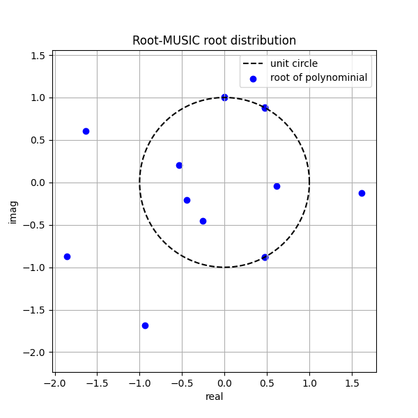
\[\sum c_i z^{(2N-2-i)} = 0 \tag{10}\]Solving Equation (10) yields \(( 2N-2 )\) roots. Since each element of the manifold vector must have unit modulus, we select the \(( N-M )\) roots that are closest to the unit circle as the corresponding \(z\) values. When plotted in the complex plane, these roots are the closest to the unit circle.
The relationship between the root angle \(\varphi\) and the beam angle \(\theta\) is given by:
\[\varphi = \frac{d 2\pi \sin \theta}{\lambda} \tag{11}\]where \(d\) is the antenna spacing, and \(\lambda\) is the wavelength.
For example, if $ d $ is half the wavelength and \(\theta = 20^\circ\), then:
\[\varphi = 61.6^\circ \times \frac{\pi}{180}\]The implementation code can be found on GitHub: https://github.com/taichiorange/leba_math, under the directory: leba_math/MIMO/MIMO-beam-detection/rootMUSIC-algorithm.py.
import numpy as np
from scipy.linalg import eigh
import matplotlib.pyplot as plt

def simulate_ula_signals(num_sensors, num_snapshots, doa_deg, d=0.5, wavelength=1.0, SNR_dB=20):
    """
    Parameters:
        num_sensors: number of sensors (antennas)
        num_snapshots: number of samples
        doa_deg: actual angles (degrees), list or numpy array
        d: distance between adjacent antennas (unit: wavelength, default 0.5, half wavelength)
        wavelength: wavelength (default is 1.0)
        SNR_dB: SNR in dB

    Returns:
        Y: array of received signals (num_sensors x num_snapshots)
    """
    doa_rad = np.deg2rad(doa_deg)
    num_sources = len(doa_deg)
    sensor_idx = np.arange(num_sensors)

    # Construct the array manifold matrix
    # Steering vector: a(θ) = [1, exp(j*2π*d*sinθ), exp(j*2π*2*d*sinθ), ...]^T
    A = np.exp(1j * 2 * np.pi * d * np.sin(doa_rad)[np.newaxis, :] * sensor_idx[:, np.newaxis] / wavelength)

    # Generate signals: complex Gaussian random signals (normalized to unit power)
    S = (np.random.randn(num_sources, num_snapshots) + 1j * np.random.randn(num_sources, num_snapshots)) / np.sqrt(2)

    # Received signals without noise
    Y_clean = A @ S  # num_sensors x num_snapshots

    # Add noise
    signal_power = np.mean(np.abs(Y_clean)**2)
    noise_power = signal_power / (10**(SNR_dB/10))
    noise = np.sqrt(noise_power/2) * (np.random.randn(num_sensors, num_snapshots) + 1j * np.random.randn(num_sensors, num_snapshots))

    Y = Y_clean + noise
    return Y

def root_music(R, num_sources, d=0.5, wavelength=1.0):
    """
    Root-MUSIC DOA estimation (for ULA).

    Parameters:
        R: sample covariance matrix of the received signals (num_sensors x num_sensors)
        num_sources: number of signals (number of DOAs to be estimated)
        d: sensor spacing (in wavelengths, default 0.5)
        wavelength: signal wavelength (default 1.0)

    Returns:
        doa_estimates_deg: estimated DOAs (in degrees, sorted in ascending order)
    """
    num_sensors = R.shape[0]

    # Perform eigenvalue decomposition of the covariance matrix
    eigvals, eigvecs = eigh(R)

    # Select the noise subspace: use the (num_sensors - num_sources) eigenvectors corresponding to the smallest eigenvalues
    En = eigvecs[:, :num_sensors - num_sources]

    # Construct the noise subspace projection matrix
    Pn = En @ En.conj().T  # Size: (num_sensors x num_sensors)

    # Extract polynomial coefficients using the Toeplitz structure:
    # For a ULA, each diagonal of Pn should theoretically be equal,
    # Here, sum the elements on each diagonal to obtain the coefficients c[k] (k from -M+1 to M-1)
    c = np.array([np.sum(np.diag(Pn, k)) for k in range(-num_sensors+1, num_sensors)])

    # Normalize: set the coefficient for k=0 (the main diagonal) to 1, which does not change the root locations
    c = c / c[num_sensors - 1]

    # Construct the polynomial coefficients; note that np.roots requires the coefficients in descending order
    poly_coeffs = c[::-1]

    # Solve for all roots of the polynomial
    roots_all = np.roots(poly_coeffs)

    # Consider only the roots inside the unit circle (theoretically, the signal-related roots should lie near the unit circle)
    roots_inside = roots_all[np.abs(roots_all) < 1]

    # Sort the roots by their distance from the unit circle and select the num_sources roots closest to the unit circle
    distances = np.abs(np.abs(roots_inside) - 1)
    sorted_indices = np.argsort(distances)
    selected_roots = roots_inside[sorted_indices][:num_sources]

    # According to theory, the phase of the root satisfies: angle(z) = -2π*d*sin(θ)/wavelength
    # beta = 2π*d/wavelength
    beta = 2 * np.pi * d / wavelength
    phi = np.angle(selected_roots)

    doa_estimates_rad = np.arcsin(phi / beta)
    doa_estimates_deg = np.rad2deg(doa_estimates_rad)

    return np.sort(doa_estimates_deg),roots_all

if __name__ == "__main__":
    # Simulation parameters
    num_sensors = 8           # Number of array sensors
    num_snapshots = 1000      # Number of snapshots; recommended to increase to improve covariance matrix estimation accuracy
    doa_true = [-20, 20, 30]   # True DOAs (in degrees)
    SNR_dB = 20               # SNR in dB
    d = 0.5                   # Sensor spacing (in wavelengths)
    wavelength = 1.0          # Wavelength

    # Generate simulated signal data (with specified beam/directions)
    Y = simulate_ula_signals(num_sensors, num_snapshots, doa_true, d, wavelength, SNR_dB)

    # Estimate the sample covariance matrix
    R = Y @ Y.conj().T / num_snapshots

    # Estimate the DOAs using the Root-MUSIC algorithm
    num_sources = len(doa_true)
    doa_est,roots_all = root_music(R, num_sources, d, wavelength)

    print("True DOAs (degrees):", doa_true)
    print("Estimated DOAs (degrees):", doa_est)

    plt.figure(figsize=(6,6))
    theta = np.linspace(0, 2*np.pi, 400)
    plt.plot(np.cos(theta), np.sin(theta), 'k--', label='unit circle')
    plt.scatter(np.real(roots_all), np.imag(roots_all), marker='o', color='b', label='roots of polynomial')
    plt.xlabel('Real')
    plt.ylabel('Imaginary')
    plt.title('Root-MUSIC Root Distribution')
    plt.axis('equal')
    plt.legend()
    plt.grid(True)
    plt.show()