lebamath
MUSIC (Multiple Signal Classification) Algorithm
MUSIC (Multiple Signal Classification) is a high-resolution spectral estimation algorithm based on subspace decomposition, commonly used in DOA (Direction of Arrival) estimation, f-k spectrum analysis, radar signal processing, etc. It utilizes the orthogonality between the signal subspace and noise subspace to distinguish different signal wave-beams k or direction angles \(\theta\), achieving super-resolution capability to resolve closely spaced wave-beams or arrival angles.
Basic Idea of MUSIC Algorithm
The MUSIC algorithm is based on the eigenvalue decomposition of the signal’s covariance matrix \(\boldsymbol R_y\), separating the signal subspace from the noise subspace. It then uses the orthogonality between the signal and noise subspaces to construct a pseudo-spectrum, and determines the signal’s wave-beams or angles through peak searching.
Steps of MUSIC Algorithm
(1) Constructing the Covariance Matrix
Assume that the received signal \(\mathbf{y}(t)\) consists of \(M\) plane wave signals and noise:
\[\mathbf y(t)=\sum_{i=1}^M s_i(t) \mathbf a(k_i)+ \mathbf n(t) \tag{1}\]where:
- \(s_i(t)\) is the amplitude of the \(i\)-th signal.
- \(\mathbf{a}(k_i)\) is the array manifold vector corresponding to the wave-beam \(k_i\).
- \(\mathbf{n}(t)\) is the noise term.
Let the number of antennas be N.
Defining:
\[\mathbf A = [\mathbf{a}(k_1), \mathbf{a}(k_2), \dots, \mathbf{a}(k_M)], \quad \mathbf S(t) = [s_1(t),s_2(t),\dots,s_M(t)]^\text T\tag{2}\]the equation above can be rewritten as:
\[\mathbf y(t)= \mathbf A \boldsymbol{S}(t) + \mathbf n(t)\tag{3}\]The spatial covariance matrix of the signal is computed as:
\[\boldsymbol R_y=\text{E}[\mathbf y \mathbf y^H]\tag{4}\]Expanding it using the previous equation:
\[\boldsymbol{R} = \text{E}\left [\left (\mathbf A \boldsymbol{S}(t) + \mathbf n(t) \right )\left (\mathbf A \boldsymbol{S}(t) + \mathbf n(t)\right )^H\right ]\tag{5}\]If the signals are stationary, and the noise is zero-mean Gaussian white noise, and signals are uncorrelated with noise, then:
\[\boldsymbol R_y=\boldsymbol A \boldsymbol R_s \boldsymbol A^H+\sigma^2 \boldsymbol I \tag{6}\]where:
- \(\mathbf A = [\mathbf{a}(k_1), \mathbf{a}(k_2), \dots, \mathbf{a}(k_M)]\) is the signal’s array manifold matrix.
- \(\boldsymbol R_s\) is the signal’s autocorrelation matrix.
- \(\sigma^2 \boldsymbol I\) is the noise covariance matrix (assuming uniform noise power).
(2) Eigenvalue Decomposition (EVD)
Perform eigenvalue decomposition on \(\boldsymbol R_y\):
\[\boldsymbol R_y = \boldsymbol U \boldsymbol\Lambda \boldsymbol U^H \tag{7}\]where:
- \(\boldsymbol U = [\boldsymbol U_s, \boldsymbol U_n]\) is the eigenvector matrix, consisting of the signal subspace \(\boldsymbol U_s\) and the noise subspace \(\boldsymbol U_n\).
- \(\boldsymbol \Lambda = \text{diag}(\lambda_1, \lambda_2, \dots, \lambda_N)\) is the eigenvalue matrix.
In this decomposition:
- The first M larger eigenvalues correspond to the signal subspace \(\boldsymbol U_s\).
- The remaining smaller eigenvalues correspond to the noise subspace \(\boldsymbol U_n\).
Thus,
\[\boldsymbol R_y = \boldsymbol U_s \boldsymbol\Lambda_s \boldsymbol U_s^H + \boldsymbol U_n \boldsymbol\Lambda_n \boldsymbol U_n^H \tag{8}\](3) Compute the MUSIC Pseudo-Spectrum
Since the noise subspace \(\boldsymbol U_n\) is orthogonal to the signal’s array manifold \(\mathbf{a}(k)\) , i.e.,
\[\boldsymbol U_n^H \mathbf{a}(k) \approx 0\tag{9}\]the MUSIC pseudo-spectrum can be constructed as:
\[P_{\text{MUSIC}}(k) = \frac{1}{\mathbf{a}^H(k) \boldsymbol U_n \boldsymbol U_n^H \mathbf{a}(k)}\tag{10}\]where:
- \(\boldsymbol U_n\) is the noise subspace eigenvector matrix.
- \(\mathbf{a}(k)\) is the array manifold vector at test wave-beam.
(4) Peak Search for Estimating Wave-beam
The MUSIC pseudo-spectrum exhibits peaks at the true wave-beams $k_i$, thus:
- By searching for the peaks of \(P_{\text{MUSIC}}(k)\) , we can determine \(k_1, k_2, \dots, k_M\).
- These peaks correspond to the real wave-beam components of the signals.
Reciprocal Structure of the Pseudo-Spectrum
- The denominator of the MUSIC pseudo-spectrum:
- If k is a true wave-beam: \(\mathbf{a}(k)\) mainly lies in the signal subspace and does not project onto the noise subspace, making the denominator approach 0, causing \(P_{\text{MUSIC}}(k)\) to reach a peak.
- If k is not a true wave-beam: \(\mathbf{a}(k)\) primarily projects onto the noise subspace, making \(\boldsymbol U_n^H \mathbf{a}(k)\) nonzero, resulting in a lower value of \(P_{\text{MUSIC}}(k)\).
✅ Therefore, MUSIC pseudo-spectrum exhibits peaks at true wave-beams!
Meaning of Eigenvalue Decomposition of the Covariance Matrix
The MUSIC algorithm aims to find the \(M\) manifold vectors \(\textbf{a}(k_i)\) from equation (1), which corresponds to finding the matrix \(\mathbf{A}\) in equation (2).
Next, we analyze equations (6) and (8).
1) Structure of the Matrix \(A R_s A^H\)
Revisiting the signal covariance matrix:
\[\boldsymbol R_y = \boldsymbol A \boldsymbol R_s \boldsymbol A^H + \sigma_n^2 \boldsymbol I\]where:
- \(\boldsymbol A\) is the \(N \times M\) array manifold matrix, with each column \(\mathbf{a}(k_i)\) being a manifold vector for a signal direction:
- \(\boldsymbol R_s\) is the \(M \times M\) signal covariance matrix, usually assumed to be diagonal:
where \(\lambda_i\) represents the power of the signal sources.
We focus on:
\[\boldsymbol A \boldsymbol R_s \boldsymbol A^H\]which is an \(N \times N\) matrix, but its rank is at most M.
2) Why is the Rank of \(\boldsymbol A \boldsymbol R_s \boldsymbol A^H\) at Most M?
(a) Basic Definition of Rank
The rank of a matrix is the number of linearly independent column vectors, i.e., the dimension of the column space.
(b) Examining the Rank of A
- A is an N×MN \times M matrix, with M columns and N rows (typically N > M).
- The column space of A is at most M-dimensional.
- Intuitively, A contains only M independent direction vectors, so its column space is at most M-dimensional.
- Assuming A is full rank, we denote rank(A) = M.
(c) After Multiplying by \(R_s\)
\[\boldsymbol A \boldsymbol R_s\]- \(R_s\) is an \(M \times M\) diagonal matrix, which does not change the rank of A (assuming all signal powers \(\lambda_i \neq 0\)).
- \(\boldsymbol A \boldsymbol R_s\) remains an N×M matrix, with its column space still spanned by A.
- Multiplying by \(\boldsymbol A^H\):
still only contains M independent directions, as it is formed by linear combinations of A.
(d) Conclusion
- \(A R_s A^H\) is an N×N matrix, but its rank is at most M, since it contains at most M linearly independent column vectors.
- In other words, \(A R_s A^H\) only contains M-dimensional signal direction information, with the remaining N−M dimensions containing only noise.
3) Why is the Column Space of \(A R_s A^H\) Spanned by A?
Since:
\[A R_s A^H = A (\text{diag}(\lambda_1, \lambda_2, ..., \lambda_M)) A^H\]Step-by-step analysis:
- \(R_s\) only scales A (since it is a diagonal matrix).
- \(A R_s\) remains within the column space of A (since \(A R_s\) is merely a scaled version of A’s column vectors).
- Multiplication by \(A^H\) only projects the space back into its original column space.
Conclusion:
Column space(\(\boldsymbol A\boldsymbol R_s\boldsymbol A^H\)) = Column space(\(\boldsymbol A\))
- The column vectors of \(A R_s A^H\) are entirely composed of linear combinations of A’s column vectors.
- Its rank does not exceed the rank of A, hence it is at most M.
4) Intuitive Understanding
You can think of \(A R_s A^H\) as a data projection process:
- A maps \(s(t)\) into N-dimensional space.
- \(R_s\) only scales, without changing direction.
- Multiplication by \(A^H\) projects the data back, keeping it in the space spanned by A.
Thus, \(A R_s A^H\) remains in the signal subspace spanned by A, and its rank is at most M.
5) Connection to the MUSIC Algorithm
(a) Signal Subspace
Perform eigenvalue decomposition on \(R_y = A R_s A^H + \sigma_n^2 I\):
\[R_y = U \Lambda U^H\]- Since \(A R_s A^H\) has only M nonzero eigenvalues, \(R_y\) also has M large eigenvalues, corresponding to the signal subspace.
- These M eigenvectors (the basis of the signal subspace) are linear combinations of A’s column vectors, since A spans the column space of \(A R_s A^H\).
(b) Noise Subspace
- The remaining N−M smaller eigenvalues of \(R_y\) are approximately \(\sigma_n^2\), corresponding to the noise subspace.
- The noise subspace eigenvectors are orthogonal to the signal subspace(please refer to next section), meaning:
This explains why the MUSIC pseudo-spectrum is constructed as:
\[P_{\text{MUSIC}}(k) = \frac{1}{\mathbf{a}^H(k) U_n U_n^H \mathbf{a}(k)}\]- At true signal directions \(k_i\), \(\mathbf{a}(k_i)\) lies in the signal subspace, causing MUSIC pseudo-spectrum to peak.
- At incorrect directions, \(\mathbf{a}(k)\) mainly projects onto the noise subspace, resulting in a lower MUSIC pseudo-spectrum value.
Explanation: Orthogonality Between Noise Subspace and Signal Subspace
1) Why Are the Noise Subspace and Signal Subspace Orthogonal?
Starting from the eigenvalue decomposition (EVD) of the covariance matrix \(R_y\):
\[R_y = U_s \Lambda_s U_s^H + U_n \Lambda_n U_n^H\]where:
- \(U_s\) is the eigenvector matrix of the signal subspace, corresponding to the largest M eigenvalues (strong signal energy).
- \(U_n\) is the eigenvector matrix of the noise subspace, corresponding to the smaller eigenvalues (typically close to the noise power \(\sigma_n^2\)).
- Since the eigenvector matrix \(U = [U_s, U_n]\) is orthogonal, \(U_s\) and \(U_n\) are mutually orthogonal.
This implies:
\[U_n^H U_s = 0\]which means the noise subspace and the signal subspace are completely orthogonal.
2) Why Are the Eigenvectors of the Noise Subspace Orthogonal to the Signal Subspace?
Since eigenvectors span a subspace, if two subspaces are orthogonal, then any vector belonging to one subspace will be orthogonal to any vector in the other subspace.
In other words:
- \(U_n\) consists of basis vectors for the noise subspace, and any linear combination of these vectors still belongs to the noise subspace.
- \(U_s\) consists of basis vectors for the signal subspace, and any linear combination of these vectors still belongs to the signal subspace.
- Since \(U_s\) and \(U_n\) are orthogonal, every eigenvector in \(U_n\) is orthogonal to every eigenvector in \(U_s\).
Thus, we can rigorously express this as:
\[U_n^H \mathbf{a}(k) \approx 0, \quad \forall k \in \text{signal directions}\]This implies:
- Any manifold vector \(\mathbf{a}(k)\) of a signal almost entirely lies in the signal subspace and does not project onto the noise subspace.
- The eigenvectors of the noise subspace are orthogonal to the signal manifold vectors, which is precisely the property utilized by the MUSIC pseudo-spectrum.
3) Summary
- The noise subspace and the signal subspace are orthogonal.
- Therefore, the eigenvectors of the noise subspace are orthogonal to all vectors in the signal subspace, including the signal manifold vectors.
- The MUSIC pseudo-spectrum exploits this orthogonality to estimate the true wave-beams or direction angles of signals.
Uniqueness of Beams in the Signal Subspace Formed by Manifold Vectors
From the previous summary, we can see that the essence of the MUSIC algorithm is to identify the noise subspace (by determining its basis) and then use the orthogonality between the signal subspace and the noise subspace to find the true manifold vectors within the signal subspace, which correspond to the actual incident beam directions.
A key question arises: within the signal subspace, which contains infinitely many vectors orthogonal to the noise subspace, how can we determine the unique true signal vectors (manifold vectors)?
We need to prove that among all manifold vectors, there exist exactly M unique vectors orthogonal to the noise subspace.
Given N receiving antennas, each manifold vector is an \(N\times 1\) column vector. Since there are M manifold vectors (corresponding to actual incident beam directions), the noise subspace has a dimension of N − M.
Since the signal subspace is M-dimensional, we use proof by contradiction to show that there exist exactly M manifold vectors orthogonal to the noise subspace.
The matrix formed by the manifold vectors is a Vandermonde matrix. When the number of column vectors is at most N, these N column vectors are linearly independent. Since M<N, any chosen M columns are also linearly independent. The signal subspace has dimension M, meaning that at most M independent manifold vectors can be found within it.
If there were M+1 manifold vectors orthogonal to the noise subspace, they would all belong to the signal subspace. However, since the signal subspace is M-dimensional, having M+1 such vectors would imply linear dependence. Yet, from the properties of the Vandermonde matrix, any M+1 column vectors (as long as \(M+1 \leq N\)) remain linearly independent, creating a contradiction. This confirms that there exist exactly M unique manifold vectors orthogonal to the noise subspace.
Vandermonde Matrix
For an \(n \times n\) Vandermonde matrix:
\[V = \begin{bmatrix} 1 & 1 & 1 & \cdots & 1 \\ \lambda_1 & \lambda_2 & \lambda_3 & \cdots & \lambda_n \\ \lambda_1^2 & \lambda_2^2 & \lambda_3^2 & \cdots & \lambda_n^2 \\ \vdots & \vdots & \vdots & \ddots & \vdots \\ \lambda_1^{n-1} & \lambda_2^{n-1} & \lambda_3^{n-1} & \cdots & \lambda_n^{n-1} \end{bmatrix}\]Its determinant is given by:
\[\det(V) = \prod_{1 \leq i < j \leq n} (\lambda_j - \lambda_i)\]- If all \(\lambda_i\) values are distinct, then the determinant is nonzero, meaning the Vandermonde matrix is full rank with rank n.
- If some \(\lambda_i\) values are identical, the determinant becomes zero, indicating the matrix is not full rank and has rank less than nn.
The matrix formed by the manifold vectors is also a Vandermonde matrix:
\[V = \begin{bmatrix} e^{j\theta_1\times0} & e^{j\theta_2\times0} & e^{j\theta_3\times0} & \cdots & e^{j\theta_n\times0} \\ e^{j\theta_1\times1} & e^{j\theta_2\times1} & e^{j\theta_3\times1} & \cdots & e^{j\theta_n\times1} \\ e^{j\theta_1\times2} & e^{j\theta_2\times2} & e^{j\theta_3\times2} & \cdots & e^{j\theta_n\times2} \\ \vdots & \vdots & \vdots & \ddots & \vdots \\ e^{j\theta_1\times(n-1)} & e^{j\theta_2\times(n-1)} & e^{j\theta_3\times(n-1)} & \cdots & e^{j\theta_n\times(n-1)} \\ \end{bmatrix}\]This can be rewritten in a form similar to the basis of a DFT transform:
\[V = \begin{bmatrix} e^{j\frac{k_1}{n\times Q}\times0} & e^{j\frac{k_2}{n\times Q}\times0} & e^{j\frac{k_3}{n\times Q}\times0} & \cdots & e^{j\frac{k_n}{n\times Q}\times0} \\ e^{j\frac{k_1}{n\times Q}\times1} & e^{j\frac{k_2}{n\times Q}\times1} & e^{j\frac{k_3}{n\times Q}\times1} & \cdots & e^{j\frac{k_n}{n\times Q}\times1} \\ e^{j\frac{k_1}{n\times Q}\times2} & e^{j\frac{k_2}{n\times Q}\times2} & e^{j\frac{k_3}{n\times Q}\times2} & \cdots & e^{j\frac{k_n}{n\times Q}\times2} \\ \vdots & \vdots & \vdots & \ddots & \vdots \\ e^{j\frac{k_1}{n\times Q}\times(n-1)} & e^{j\theta_2\times(n-1)} & e^{j\frac{k_3}{n\times Q}\times(n-1)} & \cdots & e^{j\frac{k_n}{n\times Q}\times(n-1)} \\ \end{bmatrix}\]where \(k_i<n\times Q\), and \(Q\) is any positive integer representing the oversampling factor.
The implementation code can be found on GitHub: https://github.com/taichiorange/leba_math, under the directory:
leba_math/MIMO/MIMO-beam-detection/root-MUSIC-algorithm.py
import numpy as np
import matplotlib.pyplot as plt
from scipy.linalg import eigh
# configure
N = 8 # number of antennas
M = 5 # number of beams
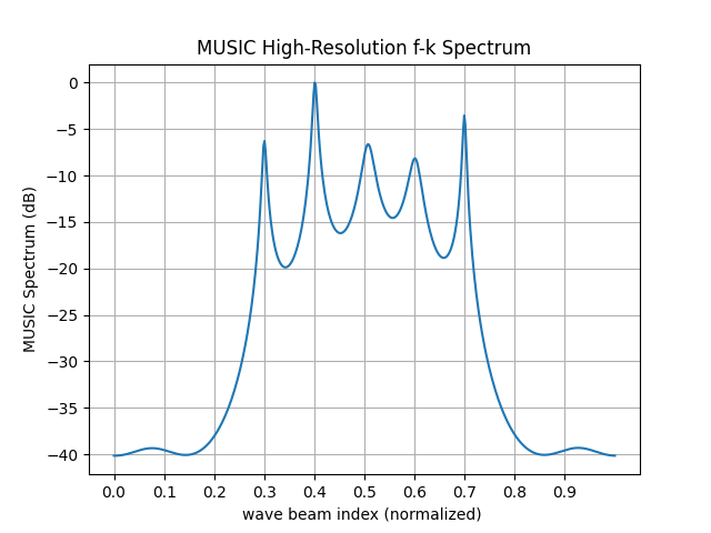
k_true = np.array([0.3, 0.4,0.5,0.6,0.7]) # beam angles
SNR = 10 # 信噪比(dB)
# create a manifold vector
def steering_vector(k, N):
n = np.arange(N)
return np.exp(1j * 2 * np.pi * k * n)
NSamples = 100
# generate signals
X = np.zeros((N, NSamples), dtype=complex)
for i in range(M):
a_k = steering_vector(k_true[i], N)
s = np.exp(1j * 2 * np.pi * np.random.rand(NSamples)) # random signals
X += np.outer(a_k, s)
# add noise
noise = (np.random.randn(N, NSamples) + 1j * np.random.randn(N, NSamples)) / np.sqrt(2)
X += noise * (10 ** (-SNR / 20))
# covariance matrix
R_y = X @ X.conj().T / X.shape[1]
# Eigenvalue Decomposition
eigvals, eigvecs = eigh(R_y)
U_n = eigvecs[:, :-M] # noise sub-space
# MUSIC pseudo-spectrum
k_scan = np.linspace(0, 1, 500)
P_music = np.zeros_like(k_scan, dtype=float)
for i, k in enumerate(k_scan):
a_k = steering_vector(k, N)
P_music[i] = 1 / np.abs(a_k.conj().T @ U_n @ U_n.conj().T @ a_k)
# normalize
P_music = 10 * np.log10(P_music / np.max(P_music))
# 绘制 MUSIC 频谱
plt.plot(k_scan, P_music)
plt.xlabel("wave beam index (normalized) ")
plt.ylabel("MUSIC Spectrum (dB)")
plt.title("MUSIC High-Resolution f-k Spectrum")
plt.grid()
plt.xticks(np.arange(0, 1, 0.1))
plt.show()